OUTTA Basic — Following the Time Axis in RNNs and Seq2Seq

Start with the hidden-state equation

I described an RNN as a repeated transformation of the current input and previous hidden state, not as a model that remembers everything. The unrolled diagram in the 38-page RNN module helped me see that parameters are shared across timesteps.

hₜ = tanh(Wₓxₜ + Wₕhₜ₋₁ + b), oₜ = Wₒhₜ + c

Batch and time axes

The first notebook check was (batch, time, feature). Without batch_first=True, the first two axes switch. A task may consume only the final timestep or pass all timestep outputs to a decoder.

Padded tokens need lengths or a mask so that they do not contribute to loss. I also checked the hidden-state shape (layers * directions, batch, hidden) when changing layer count or bidirectionality.

Train and test separate

In the retained RNN figure, training accuracy approaches 1.0 while test accuracy stays near 0.5. More epochs do not close the gap; the pattern looks like memorization rather than improved generalization.

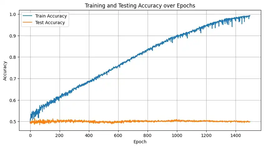
I returned to sequence length, splitting, class balance, hidden size, and dropout. Adjacent windows cut from the same source can also become overly similar when distributed across train and test.

Reading different learning curves

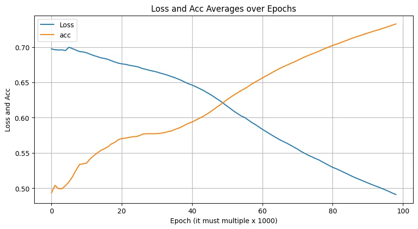
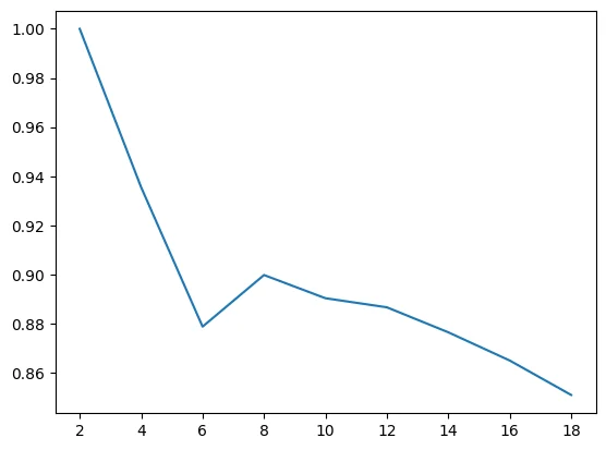
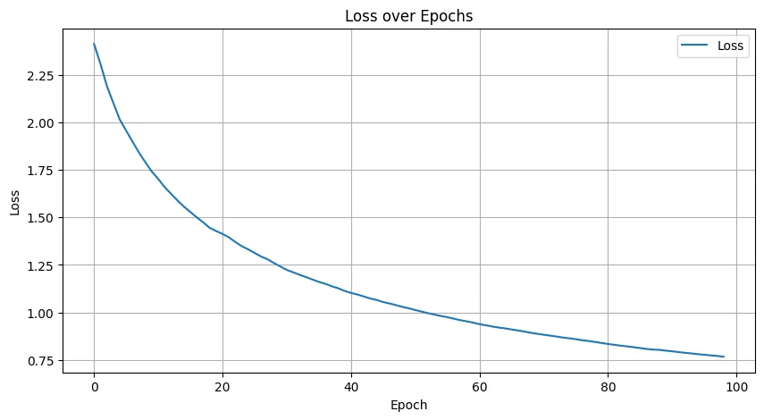
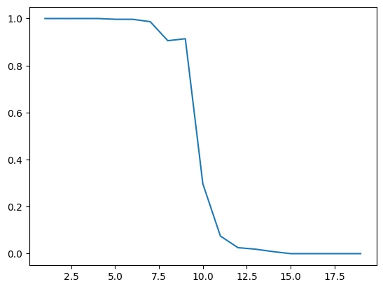
Other retained outputs showed loss decreasing while accuracy rose. A short series dipped, rebounded, and fell again; another loss curve decreased steadily. I learned to inspect the x-axis definition and sequence length before comparing plots directly.

Connecting encoder and decoder

In Seq2Seq, an encoder reads the source and a decoder begins from <bos> to produce target tokens. I initially confused all encoder outputs with the final hidden state. Without attention, the final hidden state initializes the decoder; with teacher forcing, the target token becomes the next decoder input.

L = −Σₜ log p(yₜ | y before t, x)

Minimal unpacked example

embedded = embedding(token_ids)             # (batch, time, dim)
encoder_output, hidden = encoder(embedded)

decoder_input = bos_tokens
logits = []
for target_step in range(target_length):
    step_vector = embedding(decoder_input).unsqueeze(1)
    step_output, hidden = decoder(step_vector, hidden)
    step_logits = projection(step_output[:, 0])
    logits.append(step_logits)
    decoder_input = target[:, target_step]  # teacher forcing

logits = torch.stack(logits, dim=1)         # (batch, time, vocab)

Previous and next

• Previous: Language models, embeddings, and autoencoders
• Next: Organizing BERT, Hugging Face, and Gemini safely