OUTTA Basic — Connecting Language Models, Embeddings, and Autoencoders

From tokens to probability

I defined a language model as a distribution over the next token given previous tokens, not a device that stores complete sentences. The 49-page language-model module led me through vocabulary construction, integer indices, context windows, and shifted targets.

p(w₁…wₜ) = ∏ₜ p(wₜ | w before t)

The same sentence becomes a different index sequence when the tokenizer or vocabulary changes. I therefore fixed padding and unknown-token indices and checked that embedding inputs used the long dtype.

TF-IDF and cosine similarity

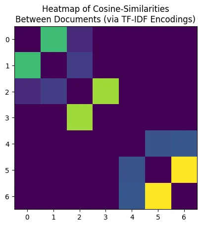
Before dense embeddings, I represented documents with TF-IDF. Cosine similarity compares direction rather than vector length. Bright cells in the heatmap connect documents with stronger vocabulary overlap.

cos(a, b) = aᵀb / (‖a‖₂‖b‖₂)

Dense embeddings

The 28-page embedding and autoencoder module replaced one-hot vectors with learned dense rows. Embedding(vocab_size, embedding_dim) appends an embedding axis to the input sequence. Cosine similarity still applies, but it now compares learned coordinates instead of raw counts.

Autoencoder latent space

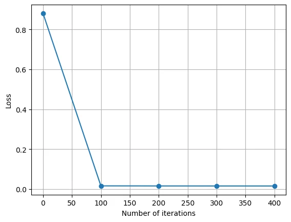
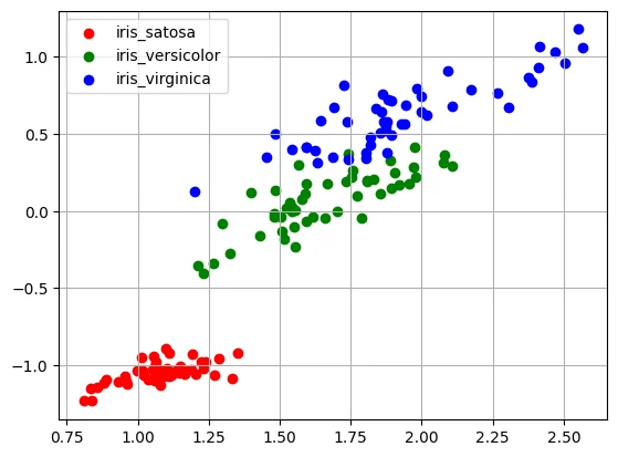
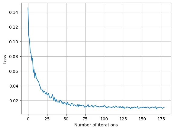
An autoencoder compresses an input into a smaller latent code and reconstructs it. I initially confused this with PCA. PCA learns linear axes; nonlinear activations between an encoder and decoder can learn a curved representation.

z = fθ(x), x̂ = gφ(z), L = ‖x − x̂‖₂²

Shape-checking code

token_ids = tokenizer(batch_text)          # (batch, time)
vectors = embedding(token_ids)             # (batch, time, dim)

latent = encoder(features)                 # (batch, latent_dim)
reconstruction = decoder(latent)           # (batch, feature_dim)

assert vectors.shape[:2] == token_ids.shape
assert reconstruction.shape == features.shape

How I compared representations

TF-IDF is easy to connect to overlapping words. An embedding stores contextual similarity in a compact dense vector. An autoencoder latent code compresses information needed for reconstruction. I treated them as tools with different objectives and interpretation methods, not as interchangeable answers.

Previous and next

• Previous: PyTorch CNN and handwritten-digit errors
• Next: Time axes in RNNs and Seq2Seq