OUTTA Basic — From Data Exploration to Autodiff and Linear Regression

Why I plotted first

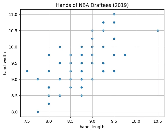
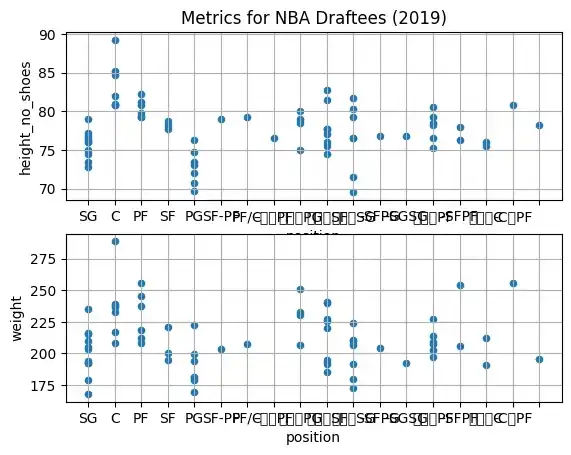
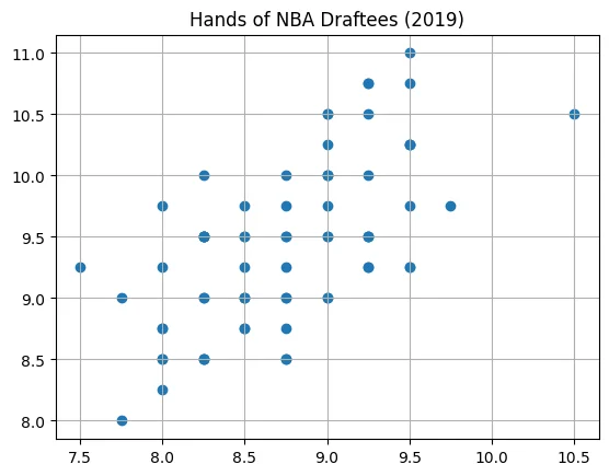
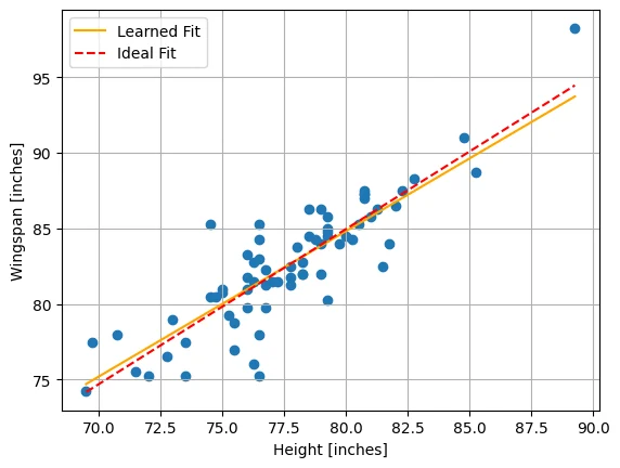
I began by plotting the inputs instead of memorizing a regression formula. After reading the 39-page regression module, I compared hand length, hand width, height, weight, and wingspan in the NBA draft measurements notebook. I checked the direction of each point cloud and noticed that a categorical axis such as position needs different handling from a continuous input.

Scatter plot of hand length and hand width for 2019 NBA draftees — Hand width generally increases with hand length.

Two scatter plots of height and weight grouped by player position — The crowded categorical labels exposed a plotting problem before modeling began.

A second hand-length and hand-width scatter plot with a simplified layout — I redrew the same relationship to check titles, axes, and ranges.

The squared function from minus ten to ten — I inspected the curvature and minimum of (x^2) before the differentiation exercise.

Reading relationships

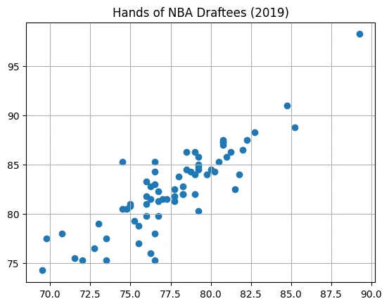
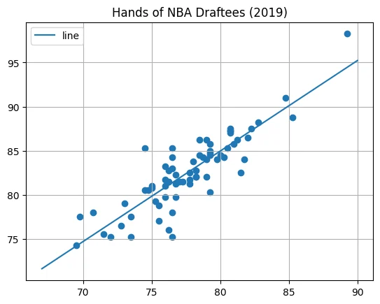
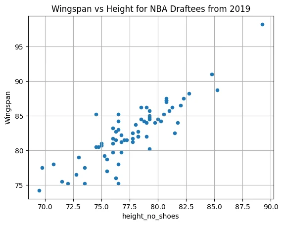
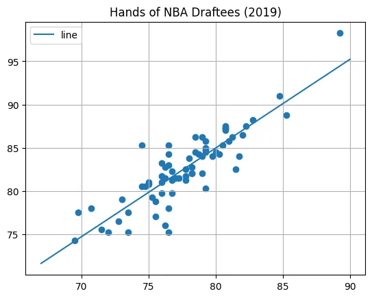
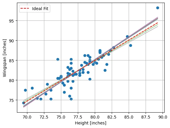
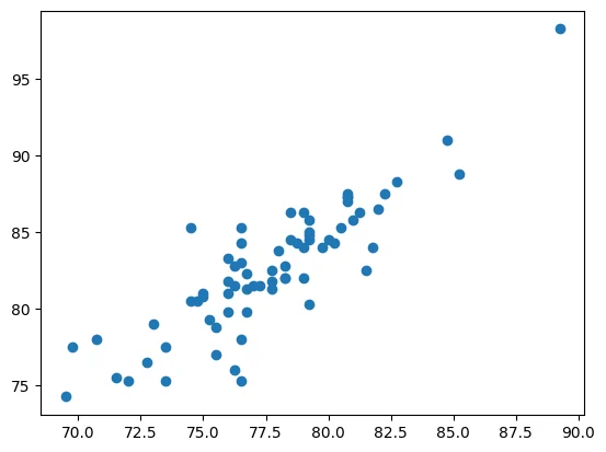
Height and wingspan showed a roughly linear relationship. I first predicted the direction from the scatter alone, then overlaid a line and repeated the plot through a second implementation. Matching axes and units mattered more than making the plot decorative.

Positive relationship between NBA player height and wingspan — I inspected direction and outliers before adding a fitted line.

First linear fit over the height and wingspan scatter — The slope and intercept place the line through the center of the point cloud.

Wingspan versus height scatter plot with explicit axis labels — The labels make the input and target roles explicit.

A second implementation of the height and wingspan regression line — Reproducing the same line cross-checked the selected columns and formula.

I wrote the model as ŷ = mx + b and the mean squared error as

L(m, b) = (1/N) Σᵢ(mxᵢ + b − yᵢ)²

Loss surfaces and autodiff

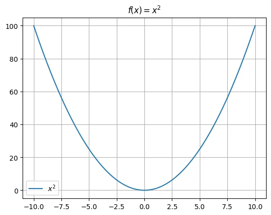
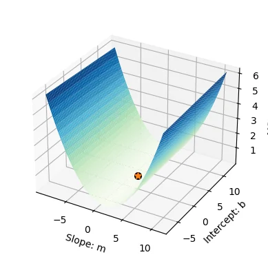
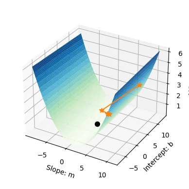
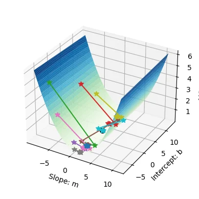
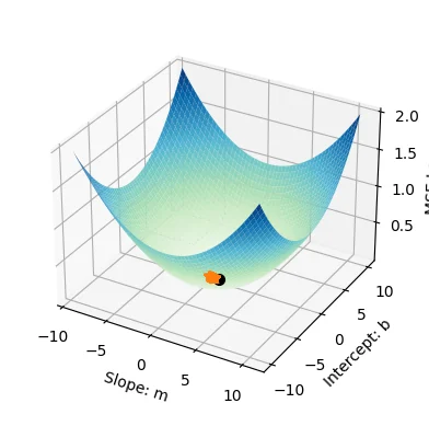
While reading the 25-page gradient-descent module, I plotted loss against (m) and (b). The phrase “move downhill” initially felt separate from loss.backward(). Marking the current point and update path on the surface connected the gradient to a direction in parameter space.

Linear-regression loss surface over slope and intercept with the current point marked — The marker locates the current parameters on the loss surface.

Loss, slope, and intercept across ten updates — A large first step reduced loss but made the parameters oscillate.

Several gradient-descent points on a regression loss surface — The updates move toward the low region of the surface.

Multiple update paths descending the same regression surface — Initialization and step size produce different paths on the same objective.

Normalization and convergence

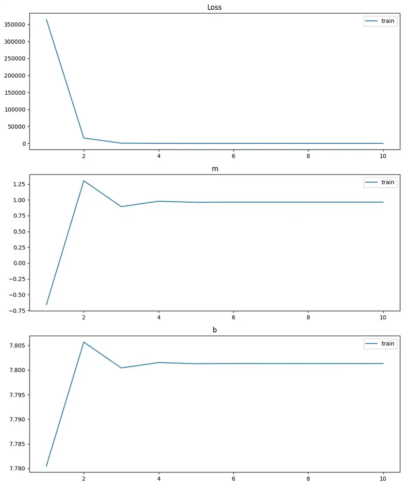
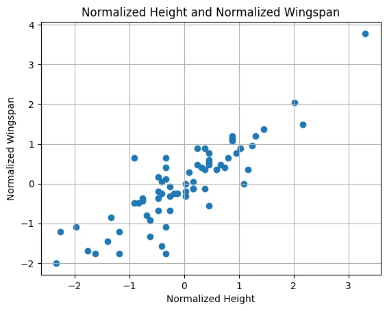
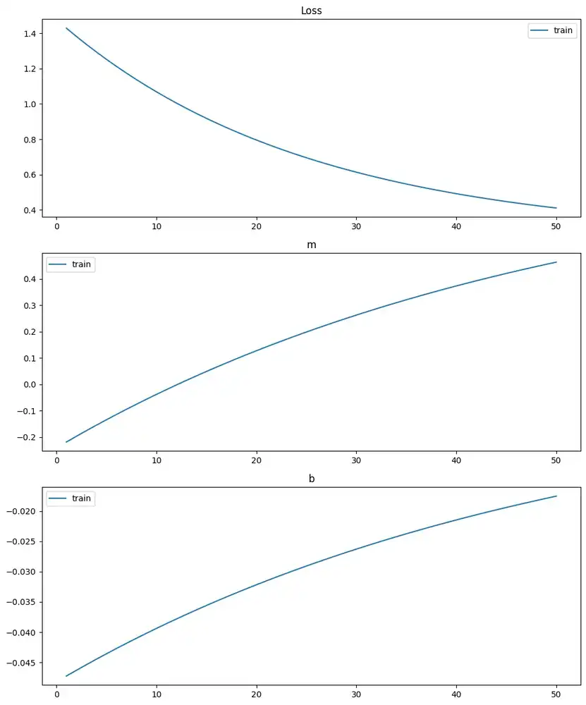
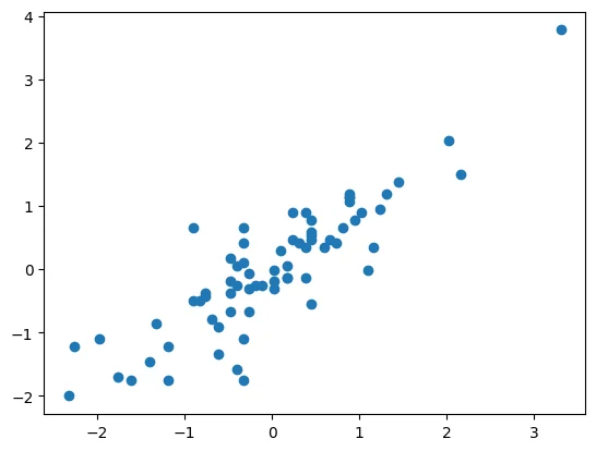
Height and wingspan scales affect gradient magnitudes. Mean subtraction and standard-deviation scaling put both inputs on comparable scales. The figures are archived notebook outputs from that exercise.

Learned and reference fits over the height and wingspan scatter — Overlaying the two lines made the slope difference visible.

Several learned regression lines and a dashed reference line — I compared whether different paths converged to similar fits.

Scatter plot of normalized height and normalized wingspan — Normalization changes coordinates without removing the relationship.

Loss, slope, and intercept stabilizing over fifty updates — After normalization, loss and both parameters settle smoothly.

Mean-squared-error surface for the normalized regression problem — The update point is easier to read around the normalized minimum.

Positive correlation between two normalized measurements — The centered coordinates preserve the positive trend.

Height and wingspan scatter restored to the original units — I returned to physical units to interpret the fitted relationship.

What stored errors taught me

My edited regression notebook retained 30 output objects, 13 figures, and three error outputs. I kept those failures in the study record and checked tensor dtype and shape, requires_grad, and the order of the update and gradient reset. Forgetting zero_grad() causes gradients to accumulate across iterations.

Minimal regression loop

m = torch.zeros((), requires_grad=True)
b = torch.zeros((), requires_grad=True)

for _ in range(50):
    prediction = m * x + b
    loss = ((prediction - y) ** 2).mean()
    loss.backward()
    with torch.no_grad():
        m -= learning_rate * m.grad
        b -= learning_rate * b.grad
        m.grad.zero_()
        b.grad.zero_()

The loop stays short but preserves forward, loss, backward, update, and reset. The next note moves from a line to function approximation and nonlinear spiral classification.

Previous: 2024 OUTTA AI Bootcamp Basic
Next: Function approximation and nonlinear classification

OUTTA Basic — From Data Exploration to Autodiff and Linear Regression

Why I plotted first

Reading relationships

Loss surfaces and autodiff

Normalization and convergence

What stored errors taught me

Minimal regression loop

Previous and next

Sources used

Why I plotted first

Reading relationships

Loss surfaces and autodiff

Normalization and convergence

What stored errors taught me

Minimal regression loop

Previous and next

Sources used

Related projects